Annoy and Approximate Nearest Neighbor Algorithm

In modern data-driven applications, finding the k nearest neighbors for a query point is a common operation. However, as datasets grow larger and dimensionality increases, the classic brute-force k-Nearest Neighbors approach often becomes prohibitively slow. This is where Approximate Nearest Neighbors (ANN) comes in—trading off a small amount of accuracy for a substantial speed-up. In this article, we will explore a popular ANN algorithm known as Annoy (Approximate Nearest Neighbors Oh Yeah), discuss how it constructs trees to speed up neighbor searches, and dive into why this “approximate” method is so powerful in practice.

Recap of k Nearest Neighbors

The k-Nearest Neighbors (kNN) algorithm is conceptually straightforward:

1. You have a training set of points.
2. A new query point $x$ arrives.
3. To classify or retrieve the k nearest points to $x$, you measure distances from $x$ to every point in the dataset and pick the closest k.

While the logic is simple, the time complexity is the key limitation. If there are nnn points in the training set, you have to compute $n$ distances. This leads to a complexity on the order of $O(n)$ for each query. For very large $n$, this quickly becomes impractical.

Moving from Exact to Approximate

Real-world applications often involve millions—even hundreds of millions—of data points. An exact nearest neighbor search for each query point can become a bottleneck. Approximate Nearest Neighbors (ANN) aims to reduce the time complexity by allowing slight inaccuracy in the results. In exchange, the retrieval is typically much faster and still good enough for many tasks, such as:

• Recommendation systems (e.g., quickly finding similar users or products)
• Natural Language Processing (e.g., retrieving similar word embeddings)
• Computer Vision (e.g., retrieving similar images based on embedding vectors)

Annoy: Approximate Nearest Neighbors Oh Yeah

One popular and easy-to-use algorithm for ANN is Annoy, developed initially by Spotify for music recommendations.

When dealing with high-dimensional data, a common strategy for nearest neighbor search is to use space-partitioning trees. Traditional methods like kd-trees or ball trees often degrade in performance when dimensions become large (the “curse of dimensionality”). Annoy’s approach is to build multiple trees that each partition the space using a simple random projection technique or we call it randomized space-partitioning tree (in fact, a forest of such trees). Here is a step-by-step explanation:

1. Random Splits:
   • Pick two random points from your dataset (say, point $\mathbf{p}_1$ and point $\mathbf{p}_2$).
   • Draw a separating hyperplane (in 2D, it’s a line; in higher dimensions, a hyperplane) that is equidistant from these two points.
   • This split divides your data into two half-spaces (region):
     • One side of the hyperplane (left half space) contains points closer to $p_1$.
     • The other side of the hyperplane (right half space) contains points closer to $p_2$.
2. Recursive Partitioning:
   • For each region, pick two random points and repeat the splitting, creating a binary tree.
   • Continue until each node (or region) has at most a small number of points (e.g., 3 to 10, depending on your chosen parameters).
3. Region Assignment:
   • The leaves of the tree each contain a small subset of points.
   • Because of how the splits are constructed, points that are close in space tend to land in the same leaf node.

Below is a placeholder for a figure showing how Annoy splits the space and how the resulting tree (or forest) looks.

Example of a Single Tree

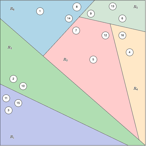
As sown in below figures, suppose you have 16 points in a 2D space. Annoy might:

• Randomly pick point #10 and point #12 to create the first split.
• Draw the perpendicular bisector (equidistant line) between them.
• Recursively continue picking pairs of random points within each partition, creating further splits, until each leaf node has at most 3 points.

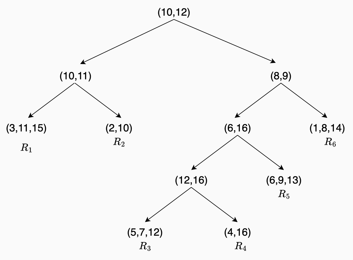
Eventually, you end up with something like this:

1. Top Node: Split the dataset using points #10 and #12.
2. Second Level: The set of points below the first line might be split using #10 and #11, while the set above might use #8 and #9, and so on.
3. Leaf Nodes: Each final region, labeled $R1, R2, \ldots$ contains only a small subset of points.

How to find a separating hyperplane ?

In a Euclidean space, the separating hyperplane (or line, in 2D) that is equidistant from two points $\mathbf{p}_1$ and $\mathbf{p}_2$ is simply the perpendicular bisector of the segment connecting those two points. Here’s the step-by-step way to construct or compute it:

1. Find the Midpoint

First, compute the midpoint $\mathbf{m}$ between the two points. If the points are given as vectors in $\mathbb{R}^d$,

This midpoint $\mathbf{m}$ is guaranteed to lie on the hyperplane you want to construct.

2. Find the Normal Vector

Compute the vector that goes from $\mathbf{p}_1$ to $\mathbf{p}_2$:

In geometric terms, this vector $\mathbf{v}$ will be perpendicular (normal) to the hyperplane. Intuitively, since the hyperplane is the “middle boundary” between the two points, its normal direction must be along the line that connects the points.

3. Form the Hyperplane Equation

A hyperplane in $\mathbb{R}^d$ can be described by all $\mathbf{x}$ satisfying

where “ $\cdot$ ” denotes the dot product.

1. $\mathbf{x} - \mathbf{m}$ is the vector from the midpoint to a generic point $\mathbf{x}$.
2. $\mathbf{v}$ is the normal vector.
3. The equation says that $(\mathbf{x}-\mathbf{m})$ is perpendicular to $\mathbf{v}$.

Because $\mathbf{m}$ is the midpoint and $\mathbf{v}$ connects the two points, any point $\mathbf{x}$ on this hyperplane is equally distant from $\mathbf{p}_1$ and $\mathbf{p}_2$.

Querying with a Single Tree

When a query point $x$ arrives:

1. Start at the top of the tree.
2. At each node, check which side of the splitting hyperplane $x$ belongs to and follow the branch.
3. Once you reach a leaf node, you only compare $x$ against the (few) points stored there.

This avoids comparing $x$ to all $n$ points and reduces the query time from $O(n)$ to roughly $O(\log n)$, assuming the tree is balanced. However, one random tree might yield sub-optimal splits, occasionally missing the true nearest neighbour—hence the term approximate.

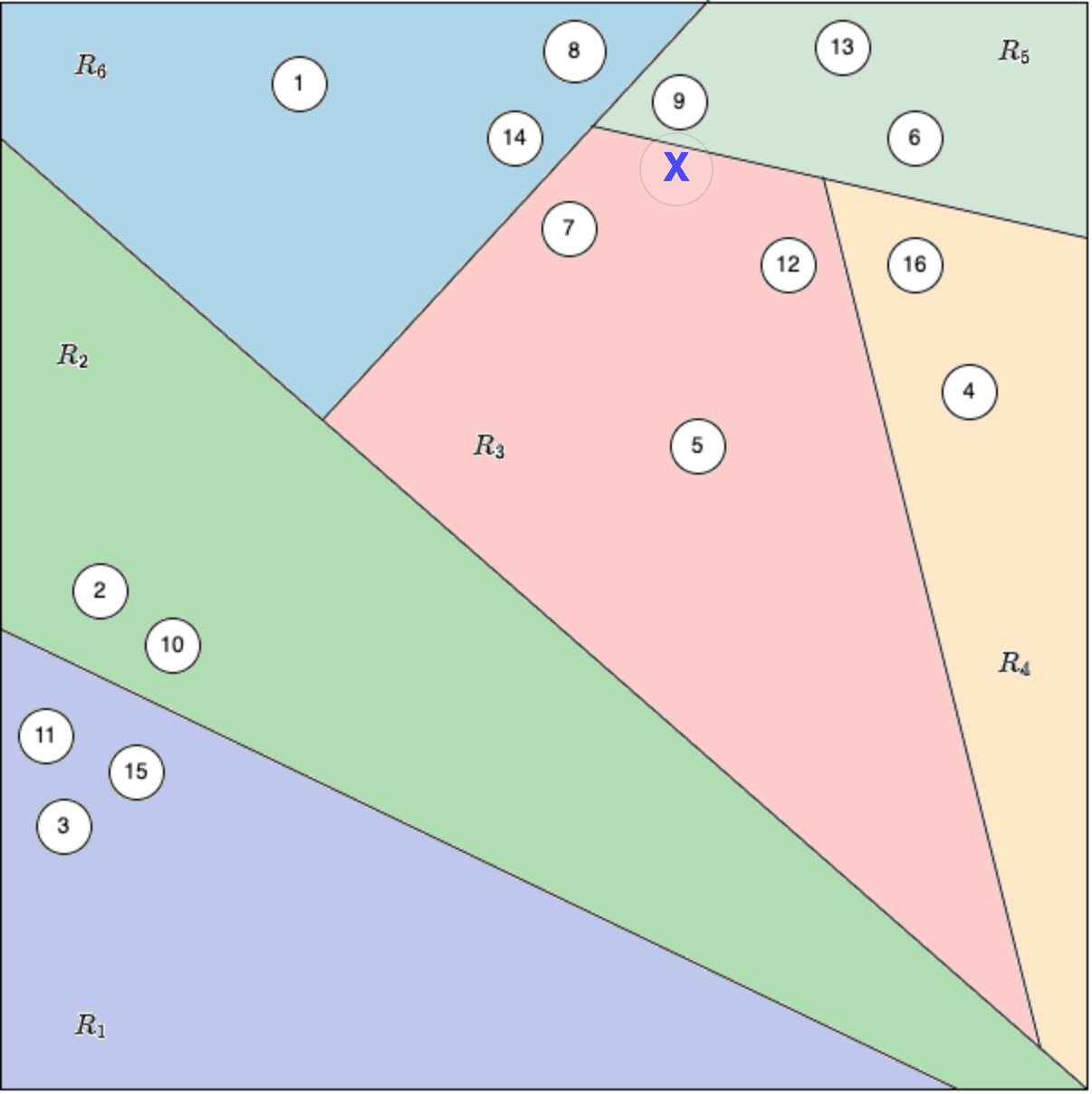
For example, consider point X in the figure below. Even though X is truly closest to point #9 in terms of distance, the random splits during tree construction may have placed X and point #9 into different regions of the tree. As a result, when we search for the nearest neighbours of X, we only look within the leaf node that X falls into and do not check across the boundary into the region containing point #9. Therefore, the search will miss point #9 as a neighbor, even though it is the closest point.

Going from One Tree to a Forest

To improve reliability and accuracy, Annoy builds multiple trees, each with different random splits:

• When searching for neighbors, Annoy searches down each tree and collects candidate neighbors from all relevant leaves.
• The final neighbor set is typically merged from candidates gathered across the forest.

This forest approach ensures that even if one tree’s random split “unluckily” separates truly close points, another tree may group them more appropriately. Searching across multiple trees increases accuracy, albeit at some additional memory cost to store all trees.

Key Trade-Offs:

1. Memory Usage: Storing more trees uses more memory.
2. Query Accuracy: More trees (and slightly deeper trees) usually increase the chance of finding the true nearest neighbors.
3. Query Speed: Each additional tree has to be traversed. However, each individual tree traversal is still $O(\log n)$.

In practice, you can tune the number of trees based on your accuracy and performance requirements. For very large datasets, building the index (i.e., constructing these trees) is a one-time cost, and subsequent queries can be extremely fast.

Why Approximate Nearest Neighbors?

Exact k-NN must scan every point—this is the only guaranteed way to find the true nearest neighbors in all cases. But when n is huge, doing $O(n)$ comparisons for every query is often infeasible.

Approximate methods sacrifice a small fraction of accuracy. However, in many real-world scenarios—especially those involving large-scale recommendation or retrieval tasks—identifying neighbors that are very close (even if not the absolute closest) is perfectly sufficient. The gains in query speed can be enormous.

Highlight of the limitations of the Annoy

Here are a few extra points not covered in the original video but worth knowing:

1. Dimensionality and Curse of Dimensionality
   • While Annoy works well in moderate dimensions (e.g., 50–1000 for embeddings), extremely high dimensions can still pose challenges for any nearest neighbor method.
   • Often, dimensionality reduction (using PCA, autoencoders, or other techniques) is applied before ANN indexing.
2. Index Building Time
   • Constructing the Annoy forest takes time proportional to $n \log n$ (since each tree is built by recursively splitting the data).
   • However, this is a one-time cost; subsequent queries are significantly faster.
3. Memory vs. Accuracy vs. Speed Trade-offs
   • The number of trees in Annoy is a critical hyperparameter. More trees can mean higher accuracy, but also more memory use and potentially slower query times if you search all of them every time.
   • Annoy also has a parameter that controls how many nodes of a tree to visit during query time (often called a “searchk” parameter), letting you tune the trade-off between speed and accuracy _at query time.

Other Popular ANN Libraries

• FAISS (Facebook AI Similarity Search): Optimized, particularly for GPUs and large-scale similarity search.
• FLANN (Fast Library for Approximate Nearest Neighbors): One of the earlier popular ANN libraries, with various indexing structures.
• HNSW (Hierarchical Navigable Small World): Graph-based approach known for high speed and recall.

Real-World Use Cases

• Music Recommendations: Spotify uses Annoy to quickly find songs or playlists similar to a user’s preferences.
• Image Similarity: E-commerce platforms use embeddings of product images to find visually similar items.
• Document / Text Search: NLP applications that embed documents or sentences into vectors can rapidly retrieve semantically similar text segments.

Building the Annoy Index

Installation

Annoy can be installed with pip:

pip install annoy

Or from source via GitHub:

git clone https://github.com/spotify/annoy.git
cd annoy
python setup.py install

Initializing and Adding Vectors

To start building an Annoy index, you need:

• The dimension of your vectors, e.g., dim = 100.
• A list of vectors you want to index (each vector has the same dimension).
• An integer index ID for each vector. This ID is used later when querying for neighbors.

Here’s a minimal example in Python:

from annoy import AnnoyIndex
import random

# Parameters
dim = 100     # dimension of your vectors
n_trees = 10  # number of trees to build in the forest

# Initialize AnnoyIndex with the dimension
# The second parameter specifies the distance metric: 'angular' is default,
# but you can choose 'euclidean', 'manhattan', etc.
annoy_index = AnnoyIndex(dim, metric='angular')

# Add vectors to the index
for i in range(1000):
    vector = [random.gauss(0, 1) for _ in range(dim)]  # random vector
    annoy_index.add_item(i, vector)

Building the Index

After adding all vectors, you build the index:

annoy_index.build(n_trees)

• n_trees: Typically, more trees result in better accuracy but longer build times and larger index sizes. A value like 10–50 is often a good starting point, depending on the size of the dataset and accuracy requirements.
• Once built, the index resides in memory.

Saving and Loading the Index

You can save the index to a file:

annoy_index.save('my_annoy_index.ann')

Later, you can load it without having to rebuild:

annoy_index_loaded = AnnoyIndex(dim, metric='angular')
annoy_index_loaded.load('my_annoy_index.ann')

This is very useful for production scenarios where you build the index offline (maybe in a batch job) and then load it for real-time queries.

Querying the Index

Getting Nearest Neighbors

To find the k nearest neighbors of a query vector, you can use:

query_vector = [random.gauss(0, 1) for _ in range(dim)]  # sample query
k = 5
neighbors = annoy_index.get_nns_by_vector(query_vector, k)

• neighbors is a list of the IDs of the nearest neighbors.