Seq2Seq Learning - An Encoder-Decoder Approach

The Encoder-Decoder architecture is widely used in sequence-to-sequence tasks, particularly in natural language processing (NLP) for tasks such as machine translation, text summarization, and image captioning. This architecture typically consists of two main components: an Encoder, which processes the input sequence and compresses it into a context vector, and a Decoder, which generates the output sequence based on this context vector. This approach enables the model to handle inputs and outputs of varying lengths, making it a powerful framework for a wide range of applications.

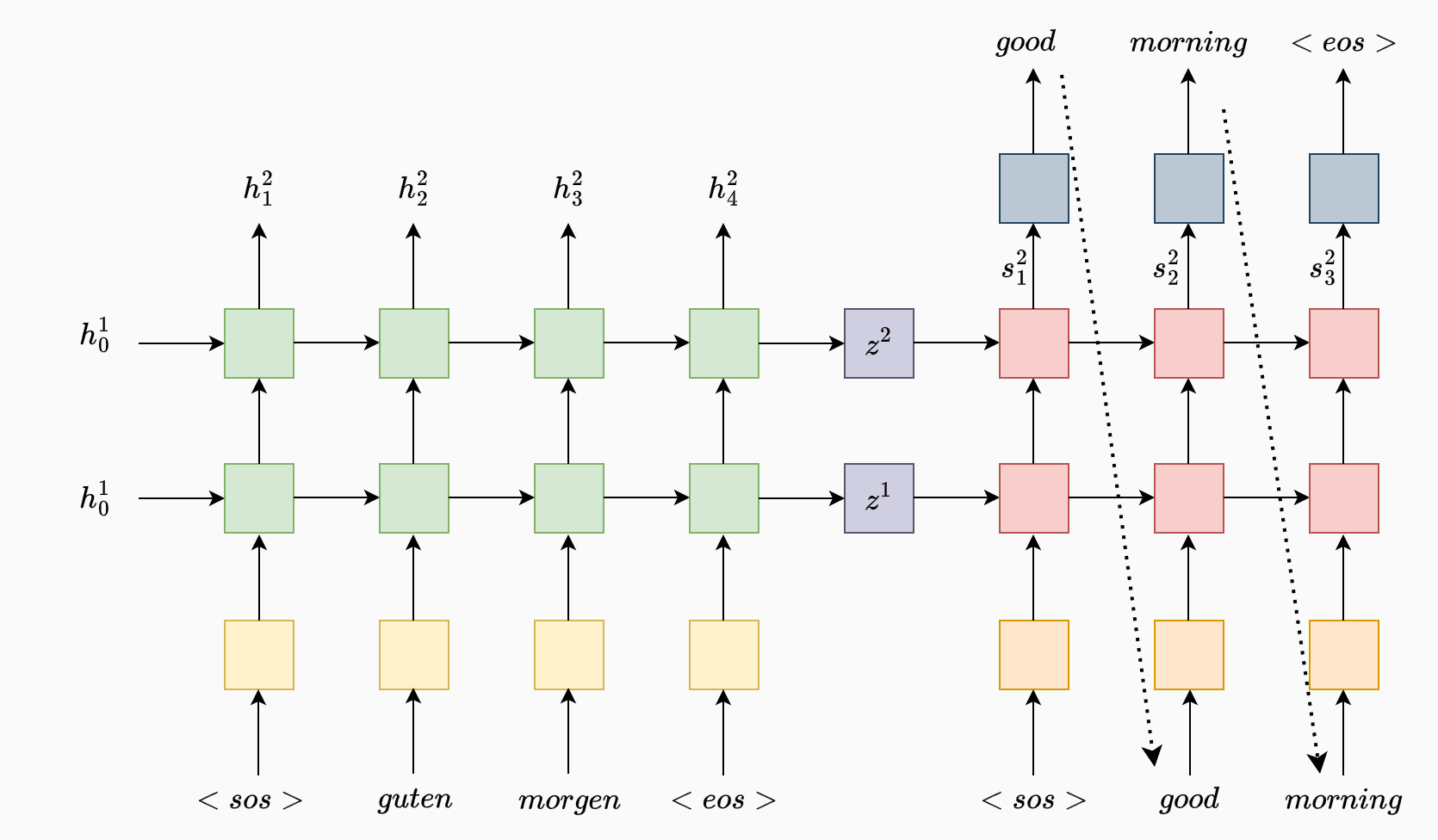
In the attached figure, the Encoder-Decoder model illustrates a machine translation task, where a sequence of words in one language (German: "guten morgen") is encoded and then decoded to generate the equivalent translation in another language (English: "good morning").

Encoder

The Encoder’s role is to process the input sequence step-by-step and summarize it into a fixed-length context vector that represents the entire sequence. In this example, each input word, including special tokens for the start (<sos>) and end (<eos>) of the sequence, is passed through an embedding layer (highlighted in yellow) and then fed into an RNN-based Encoder (green). The embedding layer converts each word into a continuous vector, allowing the model to understand relationships between words beyond their discrete token form.

At each time step $t$, the Encoder receives the embedding $e(x_t)$ of the current word and the hidden state $h_{t-1}$ from the previous time step. The Encoder RNN processes this information and outputs a new hidden state $h_t$, which can be thought of as a vector summarizing the sentence up to that point. Here we have a two-layer recurrent neural network (RNN) encoder, where each layer has its own set of hidden states to process the input sequentially.

• First Hidden Layer: The first equation represents the hidden state at the first layer, $h^{1}_t$, which is updated at each time step $t$ by the Encoder RNN. Specifically, it takes as input the encoded representation of the current input $x_t$, denoted as $e(x_t)$, and the previous hidden state $h^{1}_{t-1}$ from the first layer. This layer captures the temporal dependencies and patterns in the input sequence, gradually building a higher-level representation of the data.

  $$h^{1}_t = \text{EncoderRNN}(e(x_t), h^{1}_{t-1})$$

• Second Hidden Layer: The second equation represents the hidden state at the second layer, $h^{2}_t$, which takes as inputs the hidden state $h^{1}_{t}$ from the first layer and the previous hidden state $h^{2}_{t-1}$ from the second layer itself. This second layer further processes the output from the first layer, allowing the model to learn more complex patterns and dependencies by adding a higher level of abstraction.

  $$h^{2}_t = \text{EncoderRNN}(h^{1}_{t}, h^{2}_{t-1})$$

This recurrent process continues until the end of the input sequence, capturing both word-level information $e(x_t)$ and contextual information through the hidden states. While RNN is used as a generic term here, the architecture could utilize more complex recurrent layers, such as LSTM (Long Short-Term Memory) or GRU (Gated Recurrent Unit), to handle long-range dependencies and prevent vanishing gradients.

In this example, the input sequence $X = \{x_1, x_2, \ldots, x_T\}$ consists of tokens such as $x_1 = \text{<sos>}, x_2 = \text{guten}$ and so forth. The initial hidden state $h_0$ is often set to zeros or learned as a parameter. After the final word $x_T$ has been processed, the Encoder outputs the final hidden state $h_T = z$, which serves as the context vector for the entire sentence.

class Encoder(nn.Module):
    def __init__(self, input_dim, embedding_dim, hidden_dim, n_layers, dropout_p):
        super().__init__()
        self.embedding = nn.Embedding(input_dim, embedding_dim)
        self.rnn = nn.LSTM(embedding_dim, hidden_dim, n_layers, dropout=dropout_p)
        self.dropout = nn.Dropout(dropout_p)

    def forward(self, src):
		    # shape mentioned in comments without batch size for simplicity
        # src = [src length]
        embedded = self.dropout(self.embedding(src))
        # embedded = [src length, embedding dim]
        outputs, (hidden, cell) = self.rnn(embedded)
        # outputs = [src length, hidden dim]
        # hidden = [n layers, hidden dim] --> n layers is 2 in above figure as we have a two layers of hidden state
        # cell = [n layers, hidden dim]
        return hidden, cell

Decoder

The Decoder is responsible for generating the output sequence one token at a time, leveraging the context vector provided by the Encoder. Once the Encoder has processed the entire input sequence, the final hidden state $h_T$ (context vector $z$) is passed to the Decoder as its initial hidden state $s_0$. This initial state captures the information of the entire source sequence and provides a starting point for the Decoder to generate the target sequence.

The Decoder also operates on a token-level basis, where each token is generated based on the hidden state of the previous time step and the embedding of the previous output token. In this model, the Decoder uses a two-layer RNN with distinct hidden states at each layer to progressively process and generate each token in the target sequence.

At each time step $t$:

• The Decoder takes in the embedding of the current token $d(y_{t})$, as well as the hidden state from the previous time step $s_{t−1}$. The initial hidden state $s_0$ is set to the final hidden state of the Encoder $h_T$, providing the context for generating the target sequence.

Decoder Process with Two Layers

• First Hidden Layer: The first layer in the Decoder processes the current token embedding $d(y_{t-1})$ (embedding of the previous output token) along with the hidden state from the previous time step $s^{1}_{t-1}$ at this layer. This layer captures initial dependencies in the target sequence. $$s^{1}_t = \text{DecoderRNN}(d(y_{t-1}), s^{1}_{t-1})$$
• Second Hidden Layer: The second layer takes the output of the first layer $s^{1}_t$ and the previous hidden state $s^{2}_{t-1}$ of the second layer, creating a higher-level abstraction. This second layer enhances the Decoder's ability to understand the output sequence dependencies at a deeper level. $$s^{2}_t = \text{DecoderRNN}(s^{1}_t, s^{2}_{t-1})$$

Generating Predictions

To generate the actual word prediction $\hat{y}_t$ at each time step, we pass the hidden state $s_t$ of the final layer through a Linear layer (represented in grey in the diagram). This Linear layer transforms the hidden state into a probability distribution over the output vocabulary, allowing the model to predict the next word in the sequence:

Where $f(s_t)$ represents the Linear transformation applied to the hidden state to predict $\hat{y}_t$.

Teacher Forcing

When generating the sequence, the Decoder produces tokens one at a time. The first token is always the start-of-sequence token $<sos>$. During training, we employ a technique called teacher forcing, where we sometimes feed the actual next word $y_t$ from the target sequence instead of the model's prediction $\hat{y}_{t-1}$. This helps the model learn more effectively by correcting errors in real time. During inference, however, the model relies solely on its predictions until an end-of-sequence token $<eos>$ is generated or a specified sequence length is reached.

class Decoder(nn.Module):
    def __init__(self, output_dim, embedding_dim, hidden_dim, n_layers, dropout_p):
        super().__init__()
        self.embedding = nn.Embedding(output_dim, embedding_dim)
        self.rnn = nn.LSTM(embedding_dim, hidden_dim, n_layers, dropout=dropout_p)
        self.fc_out = nn.Linear(hidden_dim, output_dim)
        self.dropout = nn.Dropout(dropout_p)

    def forward(self, input, hidden, cell):
		    # shape mentioned in comments without batch size for simplicity
        # input shape: [1] (one token at a time)
        input = input.unsqueeze(0)  # convert to [1, 1] for batch processing
        embedded = self.dropout(self.embedding(input))
        # embedded = [1, embedding dim]

        # Pass through the RNN
        output, (hidden, cell) = self.rnn(embedded, (hidden, cell))
        # output = [1, hidden dim]
        # hidden = [n layers, hidden dim] --> n layers is 2 here for two hidden layers
        # cell = [n layers, hidden dim]

        # Prediction
        prediction = self.fc_out(output.squeeze(0))
        # prediction = [output dim]  --> target vocabulary size

        return prediction, hidden, cell

Final Seq2Seq model

The Seq2Seq class combines the Encoder and Decoder to create a complete sequence-to-sequence model. In the forward function, the source sequence (src) is first passed through the Encoder to generate initial hidden and cell states, which act as the context for the Decoder. The Decoder then processes each token in the target sequence (trg), using either the true token (with teacher forcing) or the predicted token from the previous time step as input. This process continues until the entire target sequence is generated, with predictions stored in outputs

class Seq2Seq(nn.Module):
    def __init__(self, input_dim, output_dim, embedding_dim, hidden_dim, n_layers, dropout_p, device):
        super().__init__()

        # Initialize the encoder and decoder within the Seq2Seq model
        self.encoder = Encoder(input_dim, embedding_dim, hidden_dim, n_layers, dropout_p)
        self.decoder = Decoder(output_dim, embedding_dim, hidden_dim, n_layers, dropout_p)

        self.device = device

    def forward(self, src, trg, teacher_forcing_ratio=0.5):
        # src = [src_len]
        # trg = [trg_len]

        trg_len = trg.shape[0]  # Length of target sequence
        trg_vocab_size = self.decoder.fc_out.out_features  # Target vocabulary size

        # Initialize the tensor to hold the decoder outputs
        outputs = torch.zeros(trg_len, trg_vocab_size).to(self.device)
        # outputs = [trg_len, output_dim]  (for each target token, stores probability distribution over the output vocabulary)

        # Encode the source sequence
        hidden, cell = self.encoder(src)
        # hidden = [n_layers, hidden_dim]
        # cell = [n_layers, hidden_dim]

        # Start with the <sos> token as the first input to the decoder
        input = trg[0]
        # input = [1]  (single token representing <sos> at start of decoding)

        # Decode the target sequence
        for t in range(1, trg_len):
            # Forward pass through the decoder
            prediction, hidden, cell = self.decoder(input, hidden, cell)
            # prediction = [output_dim]  (vocabulary size of output language)
            # hidden = [n_layers, hidden_dim]
            # cell = [n_layers, hidden_dim]

            # Store the output
            outputs[t] = output

            # Decide if we use teacher forcing
            teacher_force = torch.rand(1).item() < teacher_forcing_ratio
            top1 = output.argmax(0)  # Get the predicted token (index of highest probability)
            # top1 = [1] (predicted next token)

            # Choose next input for decoder
            input = trg[t] if teacher_force else top1

        return outputs

Conclusion

The Encoder-Decoder architecture has revolutionized sequence-to-sequence tasks, offering a versatile and efficient framework for handling inputs and outputs of varying lengths. By leveraging powerful components like RNNs, LSTMs, and GRUs, these models capture intricate patterns and dependencies in sequential data, enabling breakthroughs in fields like natural language processing and computer vision.

Next Steps

Attention Mechanism in Encoder - Decoder Architecture